2nd Order Active LPF Calculator Online

⚡ 2nd Order Active LPF Calculator

Sallen-Key topology · Butterworth response · Equal R, equal C assumption

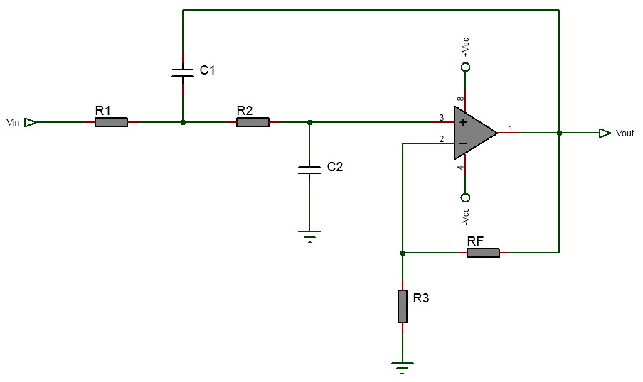
The following is an online calculator for a second order active low pass filter. The two RC stages use R₁, C₁ and R₂, C₂ respectively. The calculator assumes R₁ = R₂ = R and C₁ = C₂ = C. For a Butterworth response the passband gain A_F must be 1.586.

Inputs

f_c — Cutoff Frequency

C = C₁ = C₂ — Capacitance

A_F — Passband Gain (1.586 for Butterworth)

R₃ — Known resistor for R_F

Results

R = R₁ = R₂

R_F = R₃ · (A_F − 1)

Tip: Select C in the range 0.001 µF – 0.1 µF for best results.

Formulae Used

Equal component assumption:

R = R₁ = R₂ C = C₁ = C₂

Resistor from cutoff frequency:

R = 1 / (2π · f_c · C)

Feedback resistor:

R_F = R₃ · (A_F − 1)

General cutoff frequency:

f_c = 1 / (2π · √(R₁·R₂·C₁·C₂))

Example

The tutorial Active 2nd order LPF on breadboard shows how to use this calculator and build and test the filter.

Butterworth Response

For Butterworth response the passband gain must be 1.586, giving a maximally flat passband with no ripple.

Rolloff

The roll-off of the second order filter is −40 dB/decade — double that of a first order active LPF.

Frequency Response

An ideal LPF has instant transition from passband to stopband. A practical filter has a smooth rolloff characterised by α_max, α_min, ω_p and ω_s.

Ideal LPF frequency response

Practical LPF frequency response

Active filters using op-amps introduce insertion gain, unlike passive filters which cause insertion loss.

2nd Order Active LPF Calculator Online